Kalman

Flexible filtering and smoothing in Julia. Kalman uses DynamicIterators (an iterator protocol for dynamic data dependent and controlled processes) and GaussianDistributions (Gaussian distributions as abstraction for the uncertain state) to implement flexible online Kalman filtering.

The package provides tools to filter and smooth and conditionally sample the state space system

x[k] = Φx[k−1] + b + w[k],    w[k] ∼ N(0, Q)

y[k] = Hx[k] + v[k],    v[k] ∼ N(0, R)

How to use

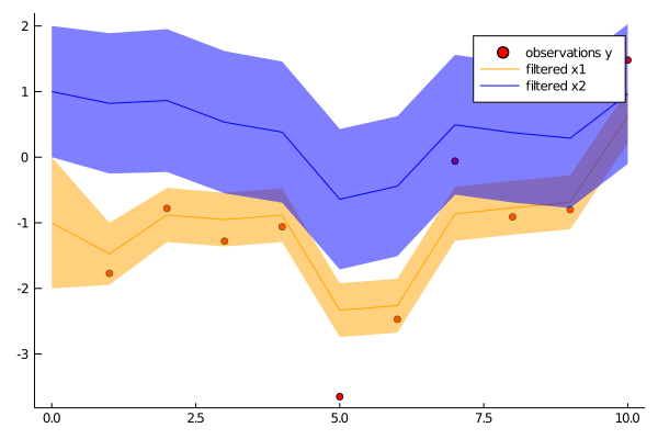
One way, and maybe the way, to use this package is to use Gaussian from GaussianDistributions.jl as representation of mean and uncertainty of a filter and call Kalman.correct to implement the correction step in a Kalman filter:

using Kalman, GaussianDistributions, LinearAlgebra
using GaussianDistributions: ⊕ # independent sum of Gaussian r.v.
using Statistics

# prior for time 0
x0 = [-1., 1.]
P0 = Matrix(1.0I, 2, 2)

# dynamics
Φ = [0.8 0.2; -0.1 0.8]
b = zeros(2)
Q = [0.2 0.0; 0.0 0.5]

# observation
H = [1.0 0.0]
R = Matrix(0.3I, 1, 1)

# (mock) data
ys = [[-1.77], [-0.78], [-1.28], [-1.06], [-3.65], [-2.47], [-0.06], [-0.91], [-0.80], [1.48]]


# filter (assuming first observation at time 1)
N = length(ys)

p = Gaussian(x0, P0)
ps = [p] # vector of filtered Gaussians
for i in 1:N
    global p
    # predict
    p = Φ*p ⊕ Gaussian(zero(x0), Q) #same as Gaussian(Φ*p.μ, Φ*p.Σ*Φ' + Q)
    # correct
    p, yres, _ = Kalman.correct(Kalman.JosephForm(), p, (Gaussian(ys[i], R), H))
    push!(ps, p) # save filtered density
end

using Plots

p1 = scatter(1:N, first.(ys), color="red", label="observations y")
plot!(p1, 0:N, [mean(p)[1] for p in ps], color="orange", label="filtered x1", grid=false, ribbon=[sqrt(cov(p)[1,1]) for p in ps], fillalpha=.5)
plot!(p1, 0:N, [mean(p)[2] for p in ps], color="blue", label="filtered x2", grid=false, ribbon=[sqrt(cov(p)[2,2]) for p in ps], fillalpha=.5)

savefig(p1, "filter.png")

A very similar example of tracking a 2D trajectory can be found here.

Interface

The same might be achieved using interface functions

using DynamicIterators, GaussianDistributions, Kalman, LinearAlgebra

# Define linear evolution
Φ = [0.8 0.5; -0.1 0.8]
b = zeros(2)
Q = [0.2 0.0; 0.0 1.0]

E = LinearEvolution(Φ, Gaussian(b, Q))

# Define observation scheme
H = [1.0 0.0]
R = Matrix(1.0I, 1, 1)

O = LinearObservation(E, H, R)

# Prior
x0 = [1., 0.]
P0 = Matrix(1.0I, 2, 2)

# Observations (mock)
Y = [1 => [1.14326], 2 => [-0.271804], 3 => [-0.00512675]]

# Filter
Xf, ll = kalmanfilter(O, 0 => Gaussian(x0, P0), Y)
@show Xf

Implementation

As said, filtering is implemented via the DynamicIterator protocol. It is worthwhile to look at a possible the implementation of kalmanfilter to see how filtering can be integrated into online algorithms (run in a local scope to avoid UndefVarError: ystate not defined.)

# `Y` is the data iterator, iterating over pairs of  `t => v` of time `t` and observation `v`
# `O` is the dynamical filter iterator, iterating over pairs `t => u` where
#     u::Tuple{<:Gaussian,<:Gaussian,Float64}
# is the tuple of filtered state, the predicted state and the log likelihood

# Initialise data iterator

ϕ = iterate(Y)
ϕ === nothing && error("no observations")
(t, v), ystate = ϕ

# Initialise dynamical filter with first data point `t => v`
# and the `prior::Pair{Int,<:Gaussian}`, a pair of initial time and initial state
prior = 0 => Gaussian(x0, P0)

ϕ = dyniterate(O, Start(Kalman.Filter(prior, 0.0)), t => v)
ϕ === nothing && error("no observations")
(t, u), state = ϕ

X = [t => u[1]]
while true

    # Advance data iterator
    
    ϕ = iterate(Y, ystate)
    ϕ === nothing && break
    (t, v), ystate = ϕ

    # Advance filter with new data `t => v`
    
    ϕ = dyniterate(O, state, t => v)
    ϕ === nothing && break
    (t, u), state = ϕ
    
    # Do something with the result `t => u` (here: saving it)
    
    push!(X, t => u[1]) # save filtered state
end
ll = u[3] # likelihood
@show  X, ll